Image processing


Indices
Check the index !
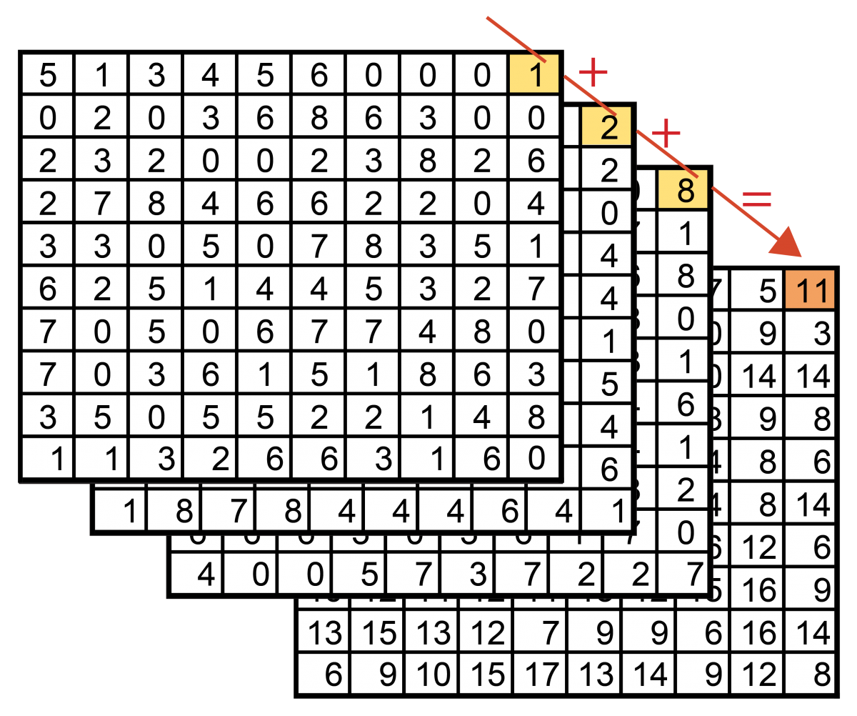
The fact that the data used in remote sensing are digital makes them most suitable for operations between channels. The principle of such operations is to perform more or less complex mathematical operations on each pixel that call upon the numerical values seen for the pixel in the various spectral bands.
For example, we can calculate the sum of the spectral values of a three-component image by doing the computation for each pixel, then storing the results in a digital image having the same number of pixels as the original image. In some cases, the result of these operations may be negative or exceed 255, which is the highest value that an image-processing system can handle. To get around these problems we can use multiplicative coefficients and/or add a constant. For example, if components A and B each vary between 0 and 255, then C = (A-B) x 0.5 + 127 will definitely be a compromise between 0 and 255.
Here, for example, is the result of applying the operation ‘red - (255 - green)’ to the picture of the Ariane 5 rocket lift-off. 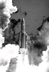
A very large number of indices of various degrees of sophistication have been developed specifically for analysing remote sensing data. One of the best known is the vegetation index. In its most widely used form, the Normalised Difference Vegetation Index, it is computed as follows:
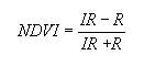
Where IR: pixel’s value in the near- infrared channel and R: pixel’s value in the red channel
To understand the principle of this index, you must remember that vegetation has a very singular spectral signature, for it exhibits a very marked peak in the near-infrared band and less reflectance in the red band.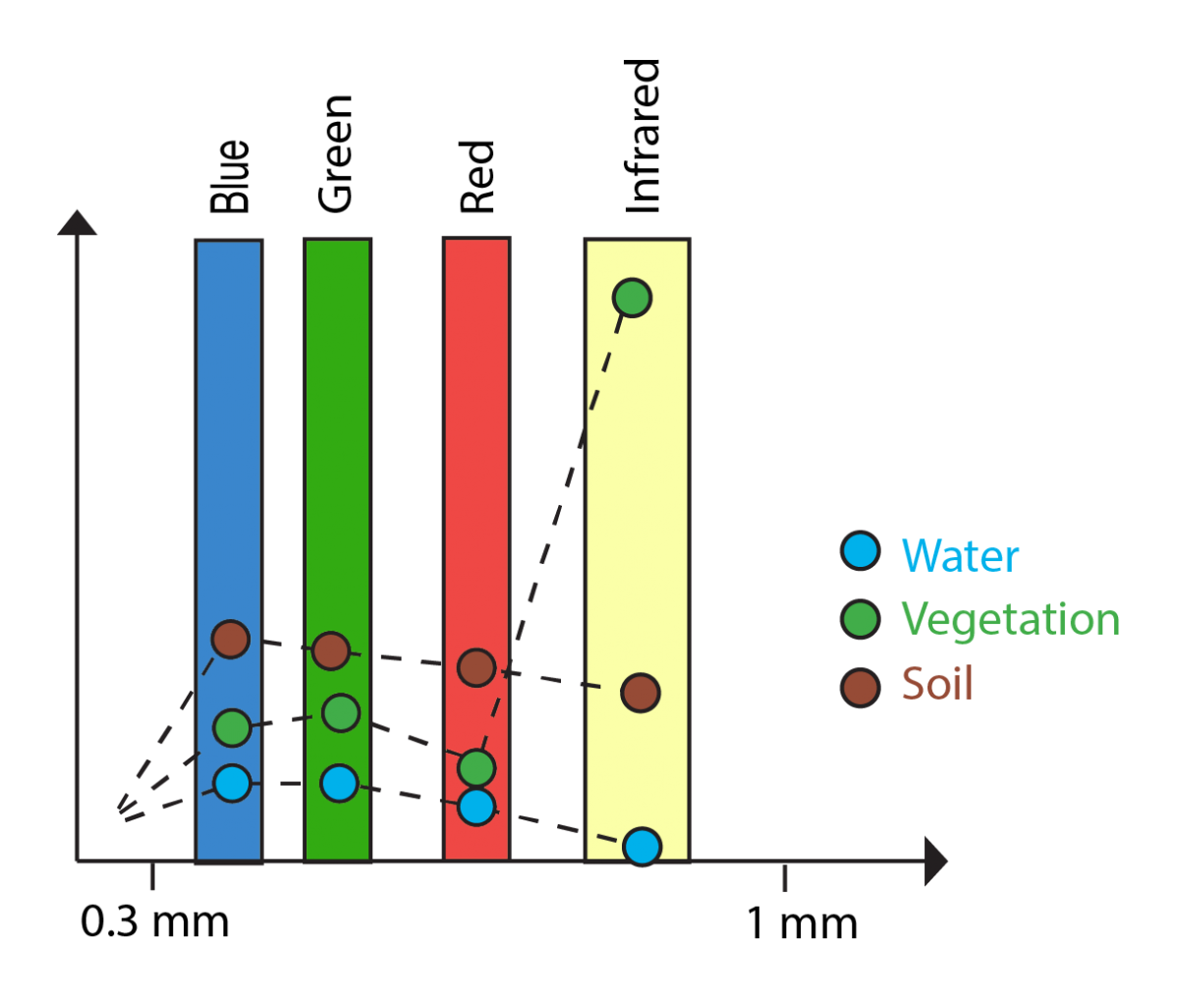
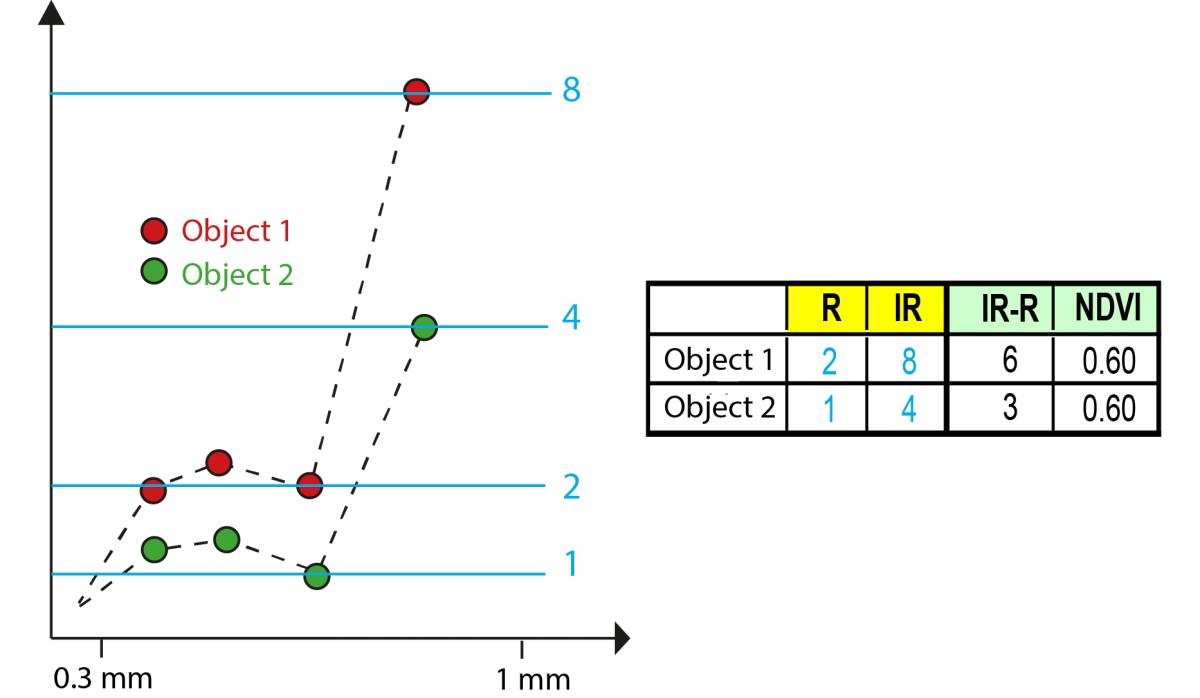
The denominator in the formula reduces the effect of differential lighting. Thus, a given object’s spectral signature will keep the same overall appearance but be shifted upward when the object is better lit (object 1).
The calculation of the simple difference IR-R is very sensitive to the difference in overall lighting whereas the normalised difference is constant.
This index is a very effective way to determine the presence of vegetation, but can also be used to estimate plant biomass and the intensity of photosynthetic activity
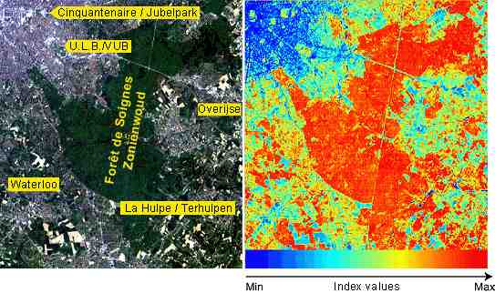
In the example below we used a Thematic Mapper image of the south-eastern part of Brussels and its outskirts. The picture on the left gives the spatial references and the one on the right corresponds to the (normalised) vegetation index calculated from the TM4 (near-infrared) and TM3 (red) bands. To make the picture easier to read, we have displayed it in pseudocolours ranging from blue for the low vegetation index values to red for the highest vegetation index values. The colour gradient at the bottom of the picture shows the gradation of colours used for this representation.
The upper left-hand corner of the image corresponds to the densely settled south-eastern part of Brussels (borough of Etterbeek). The vegetation index for this borough as a whole, which is composed for the most part of buildings and roads, is very low. However, the Jubilee Park, wooded ULB-VUB university campus and Woluwe Park stand out remarkably well on the vegetation index image, looking like so many ‘green islands’ in an urban sea. The forest (Zonienwoud/Forêt de Soignes) logically shows up as a large area of vegetation with high vegetation index values.
The other areas with high vegetation indices correspond to smaller woods and pastures, meadows and grasslands (south of Waterloo and La Hulpe). The bodies of water studding La Hulpe (Genval Lake, etc.) show up remarkably well because of their very low vegetation indices, whereas it is rather difficult to spot them in the picture on the left (‘true colour’ coloured composition).