Image processing


Supervised classification
Monospectral tresholding
In some cases it is possible to isolate a category of objects by applying thresholds to the numerical values in a single spectral band (this technique is called monospectral thresholding). This is done fairly often for aquatic surfaces seen via a near-infrared sensor, that is, all of the pixels whose numerical values are below a threshold value can be assigned to the ‘water’ class. In some cases, an object class will be defined by a range of values (‘all of the pixels whose numerical values are between 56 and 87 are classified as broad-leaf forest’, for example). This type of thresholding is often represented graphically on the histogram of the image’s numerical values. The threshold values are usually set interactively.
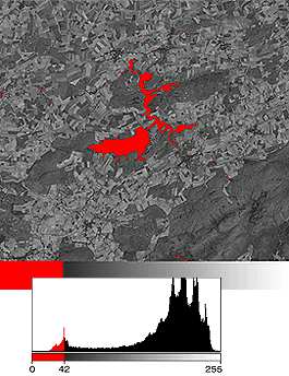
In this example, interactive thresholding in the TM4 band, covering the near-infrared band, was applied to the image of the Eau d’Heure lake. The pixels whose values are below 42 are grouped into one class that is displayed in red overlay. This type of thresholding is fairly effective, even though some ‘stray’ pixels may be seen. Unfortunately, in most cases this method can be used for the ‘water’ class only.
Multispectral tresholding
... or boxing it up
If you have several spectral bands to work with, it is also possible to do thresholding jointly in each of the bands. To visual the principle of this classification, called multispectral thresholding or box classification, a special form of histogram, called a scattergram or dispersion diagram, is used. These scattergrams can show the distribution of an image’s spectral values in two spectral bands at once:
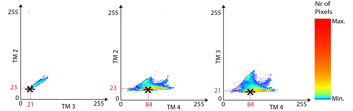
The horizontal axis of the left-hand graph represents the numerical values in the TM3 band (from 0 to 255), and the vertical axis corresponds to the values observed in the TM2 band. The point marked by a star (*) thus corresponds to the combined values of 21 in TM3 and 23 in TM2. By convention, the colour of this point in the scattergram is proportional to the number of pixels in the image that have both the value of 21 in the TM3 band and the value of 23 in the TM2 band. This is thus a graph that shows the number of pixels having a given numerical value. The area defined by these two axes is called a two-dimensional ‘spectral space’. If you want to describe an image composed of more than two spectral bands, you have to use several scattergrams (band 1/band 2, band 2/band 3, band 1/band 3). Here we see that the point marked by a star has the following spectral value: TM2 = 23, TM3 = 21, and TM4 = 84. The scattergram’s orange-red colour at this point indicates that this spectral signature is very frequent in the image.
When data with three spectral bands are analysed, the analogy that immediately comes to mind is that of a three-dimensional cloud of points seen through the three faces of a cube. The numerical values taken by a pixel in each of the n spectral bands can be considered co-ordinates in an n-dimensional system. A pixel will thus correspond to a point in n-dimensional space, sometimes called a "spectral vector".
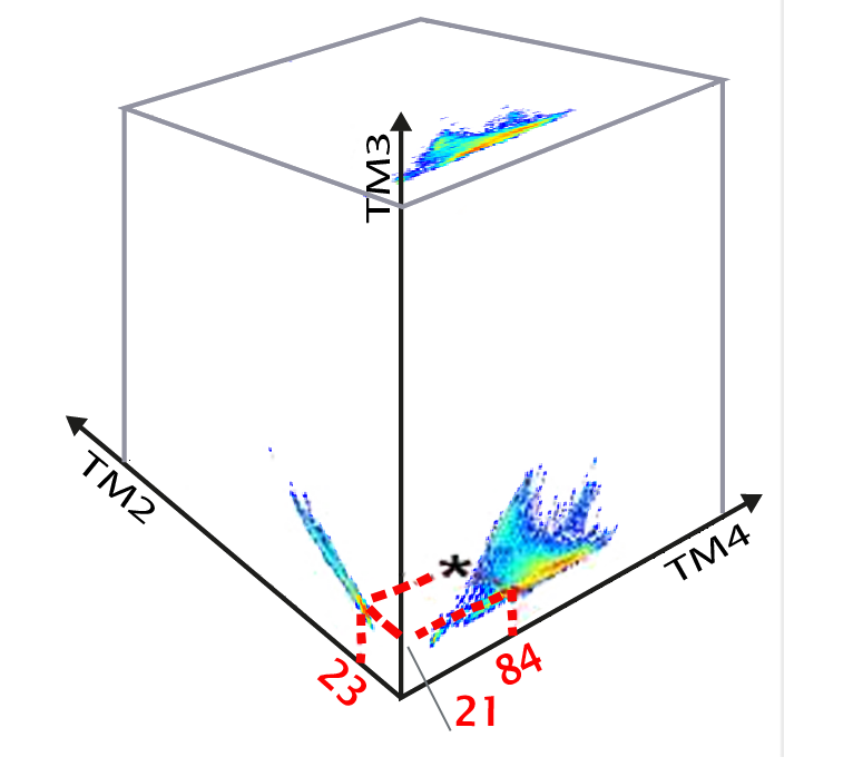 In applying a value threshold to a spectral band we define the minimum and maximum values corresponding to a type of object. Defining the maximum and minimum thresholds jointly on two spectral bands will define a rectangular area in the corresponding scattergram. If we add thresholds in the third band, we define a parallelepiped in the cloud of points. If we repeat this operation for each object class we will define a series of parallelepipeds or ‘boxes’ in this three-dimensional spectral space, hence the term box classification. It is obviously possible to set thresholds in spectral spaces with more than three dimensions, but the physical analogy then becomes more abstract.
Setting (for each object class) the minimum and maximum thresholds in each spectral band is related to a decision rule. Once the decision rule is set, the spectral values of each pixel in the image are compared with the thresholds set in the multispectral space, and if the pixel’s numerical values meet all the tests corresponding to a class, then the pixel is assigned to that class.
Implementing such a classification calls for a training phase, in which the interpreter defines in the image areas for which he knows the type of cover. The thresholds above and below each of the classes are set in relation to these sample areas. This is the phase in which the decision rule is worked out, based on analysis of a sample, and which justifies the name ‘supervised classification’ that is given to this method. (Actually, monospectral thresholding can also be considered a rudimentary form of supervised classification.)
Minimum distance classification
Why go so far?
The principle of classification by minimum distance is not fundamentally different from that of thresholding. Here, too, the decision rule’s properties are defined according to the spectral characteristics of the sample areas that have been chosen as representative of the various object classes. The minimum and maximum thresholds used for the preceding method defined parallelepipeds (‘boxes’) in multispectral space. In this method, each class’s ‘centre of gravity’ is defined and the spectral vectors corresponding to the image’s pixels are assigned to the class with the closest centre of gravity.
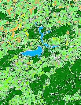
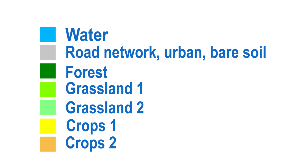
In the example shown here, we have a water class (in blue), one type of forest (in dark green), two types of grassland (in light green), and two types of crops (yellow and orange). It is not possible to differentiate among built areas, roads, and certain areas of bare ground (in grey).
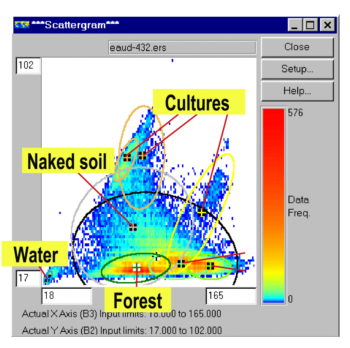
In a two-dimensional spectral space the areas defined by such a decision rule are ellipses. In a three-dimensional space it will define ellipsoid volumes, and so on.
The TM4 and TM3 band scattergram on the right shows the ellipses that are generated by such a classification.
You can see that some classes, such as water, forest, grasslands, and certain crops are well defined spectrally (small ellipses), whereas others encompass very different spectral signatures (crops, bare soil).
This suggests that new subclasses with more homogeneous spectral properties must be defined.
Maximum likehood classification
It's probably a forest !
Classification by maximum likelihood is not very different from the minimum-distance classification method. It also uses sample areas to determine the object classes’ characteristics, which then also become centres in multispectral space. In contrast, instead of assigning a spectral vector to the class with the closest centre of gravity, maximum-likelihood classification is based on statistical analysis of the distribution of the sample’s spectral vectors to define equivalent probability areas around these centres. The probabilities of each vector’s belonging to each of the classes are calculated and the vector is assigned to the class for which this probability is the highest. This method has the considerable advantage of providing an index of certainty linked to the choice for each pixel, in addition to the class to which it is assigned. It is thus possible to process the pixels classified as ‘forest’ with more than 90% certainty differently than the pixels classified as ‘forest’ with low probability. For example, there will be less hesitation about reassigning the latter to another class during subsequent processing. As interesting as this possibility may be, it nevertheless is used very seldom by most remote-sensing data software.
Post-supervised classification
... or 'fine tuning'
All of the methods outlined above assume that an interpreter can define the examples that correspond to each of the object classes that one wants to identify. In practice, we find that to get good results you generally have to define several subclasses of objects that have slightly different spectral properties, even if all of the pixels classified in these subclasses have to be put back into a single category after classification. For example, the spectral properties of broad-leaf forests often vary noticeably according to the slope’s exposure. If broad-leaf forests are broken down into three subclasses, ‘broad-leaf forest on a southern slope’, ‘broad-leaf forest on a shady slope’ and ‘broad-leaf forest on a plateau’, the classes’ spectral definitions become much more precise. This in turn improves the quality of the classification considerably. The trade-off is a more complex classification procedure (more sample areas must be selected).
If we take this reasoning one step farther, we could end up with a very large number of classes without truly worrying about their types. This can be done by algorithms that detect ‘natural’ groups of spectral vectors in the images. The interpretation work is then done after the classification, when the operator will have to assign a class to each of the groups of pixels identified in the unsupervised phase. This approach has the advantage of being able to allow for the distribution of pixels belonging to a given group of spectral signatures in the identification phase. This is not possible using the other methods.